Synchronization is a fascinating fundamental physical effect which can be observed in many different systems, ranging from biology to physics and even human behavior. It was first described by Huygens in the 18th century, when he observed that pendulum clocks hanging on a wooden beam started to swing in unison.
Systems where synchronization can appear have to have the following properties:
Individual parts, which have their own, individual behavior. The individual pendulum clocks are an example and we call this the dissimilarity of the system.
A coupling mechanism, which connects the parts and aligns their motion. In the Huygens example, this is the wooden beam which connects the clocks.
Synchronization only appears if the coupling mechanism is stronger then the tendency of each part to evolve at their own. It can be understood was the fact that the coupling strength has to overcome the dissimilarity of the system.
We say that synchronization happens if the two following conditions are observed:
All oscillators rotate with a common frequency.
The angular differences between the oscillators are bounded.
To study synchronization, we need to establish mathematical models which can describe a system with the properties described in the previous section. The possibly simplest system is the so called Kuramoto model. Here, we describe each part by an oscillators which rotates around a circle. In the classical model, all oscillators are connected to each other, but we allow the oscillators connected by a general network. The following can be observed:
The strength of the coupling depends on a coupling value and the structure of the network. In the following applet, the coupling strength and the network can be changed. The oscillators rotate on the circle on the left. The right panel shows the so called order parameter. A large value corresponds to a synchronized state.
We denote each part \(i\) by its position on a circle (which corresponds to the angle \(\theta_i\), from \(0^{\circ}\) to \(360^{\circ}\), which rotates with its own frequency \(\omega_i\). Without any coupling, the angle at time \(t\) can be calculated as \(\theta_i(t) = \omega_i t + \theta_i(0)\). The coupling between each part is described by the sinus of the angle difference. The matrix \(A\) describes which oscillator is connected to each other. In the classical Kuramoto model, this matrix is identical to one everywhere.
The full systems equation is given by:
\[\begin{aligned} \frac{d\theta_i}{d t} = \omega_i - \frac{K}{N} \sum_j \sin A_{ij} \left( \theta_i - \theta_j\right)\end{aligned}\]
Where \( \frac{d\theta_i}{d t}\) describes change in time of the variable \(\theta_i\). For identical angles \(\theta_i\), the sinus term is zero and the system evolve in synchronized manner, similar as described before.
An interesting video about synchronizations in metronomes (closely related to Huygens pendulum clocks!) can be seen here:
A good example for synchronization is the two oscillator system. Under some assumptions, we can study the evolution of the angular differences between the oscillators. If the differences of the angles is constant, the angular frequency of both oscillators has to be identical and their distance is bound, e.g. we have synchronization.
If we assume that both oscillators have the same natural frequency but rotate in opposite directions, we can express a formula for the angular difference, denoted here as \(\Delta \theta\).
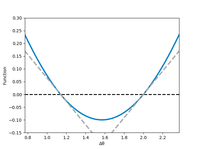
We can study the resulting formula for the evolution of the angular difference for different couplings. We are interested in where the formula is zero: Here, the angular differences between the oscillator does not change. In the following applet, the coupling between the oscillators can be changed. Try to find where this is the case!
As we can see, we need a minimum value of the coupling to observe synchronization. Systems with smaller coupling will not synchronize and the oscillators will rotate relatively freely. Finding conditions for synchronization is a sometimes difficult and interesting research task!
Another important observation is that synchronization can happen for two different values of the angular difference! We call this values the equilibrium points of the system. So, what happens in the system?
As it turns out, one of this equilibrium points is stable, while the other point is unstable. We can picture stability by the behavior of a rolling ball in a very hilly environment1, as illustrated in the following drawing:

Both rolling balls are sitting still on their reflective point, but will show very different behavior when exposed to a small force:
Ball A will roll down to one side of the mountain and never return to its original point.
Ball B will roll back and forth over its original point. With friction, it will eventually slow down and come to a still at the original point.
A similar behavior is found in the system. We call the original point of ball B stable, while ball A’s is unstable. We find out whether an equilibrium point is stable by investigating the behavior around the zero crossing:

For the left equilibrium point, the function is positive on the left side of the equilibrium point and negative on the right side. For the other equilibrium point, this is reversed. The sign of the function shows us in which direction the angular difference will evolve. So, for the right equilibrium point, angular differences larger then the equilibrium point will shrink, will smaller will increase. This corresponds to the stable solution, as small deviations from the equilibrium point will be corrected. For the other point, the opposite is true. Too large differences will increase further and too small differences decrease. This is unstable, as the same, small deviations will grow automatically.
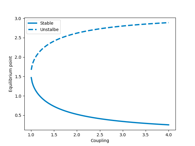
As observed before, the number of equilibrium points changes depending on the coupling strength. This qualitative change in behavior is called a bifurcation. Bifurcations are an important behavior in many dynamical systems and have been studied extensively in chaos theory, as they are closely linked to the emergence of chaotic behavior. Bifurcations are often studied by their bifurcation diagram, which shows the equilibrium points with respect to a variable. The bifurcation diagram with respect to the coupling strength looks like this:

The observed bifurcation is also called a Saddle-node bifurcation.
Here, we formalize the argumentation about equilibrium points and stability of the previous chapter, for the interested reader:
We describe a dynamical system by its state variables \(x\) (in general, a vector). An important feature of dynamical systems is that their behavior only depend on the current state. Continuous dynamical systems are usually described by a set of (ordinary) differential equations, given as: \[\begin{aligned} \frac{d}{dt} x = f(x)\end{aligned}\]
Often, their behavior is studied by the equilibrium points \(x^*\), which are the solution of: \[\begin{aligned} f(x^*) = 0\end{aligned}\]
We investigate the stability by investigating the behavior of a vector \(x = x^* + \Delta x\), with a small pertubation \(\Delta x\). We assume that \(\Delta x\) is positive, the same argument can be made for negative \(\Delta x\) (with inverted signs).
We can then study the behavior by Taylor-expanding \(f\) and get: \[\begin{aligned} f(x) \approx \underbrace{f(x^*)}_{=0} + \sum_j \underbrace{\frac{\partial f(x^*)}{\partial x_j}}_{=J} \underbrace{\left( x_j - x_j^* \right)}_{=\Delta x_j} \\ \text{With the Jacobian matrix: } J = \begin{pmatrix} \frac{\partial f_1}{\partial x_1} &\dots & \frac{\partial f_1}{\partial x_n} \\ \vdots & \ddots & \vdots \\ \frac{\partial f_n}{\partial x_1} &\dots & \frac{\partial f_n}{\partial x_n} \end{pmatrix}\end{aligned}\]
We can then calculate the stability by the eigenvalues of the Jacobian matrix at the fixed point (\(J(x^*)\)). Negative eigenvalues correspond to stable fixed points.
We try to calculate a critical value for the existence of a synchronized solution of the Kuramoto model. As before, the phases of the Kuramoto model is given as:
\[\begin{aligned} \frac{d\theta_i}{d t} = \omega_i - \frac{K}{N} \sum_j \sin \left( \theta_i - \theta_j\right)\end{aligned}\]
We define the order parameter \(r\) and the average phase \(\psi\) with the imaginary unit \(i = \sqrt{-1}\) as:
\[\begin{aligned} r e^{i\psi} = \frac{1}{N} \sum_j e^{i \theta_j}\end{aligned}\]
If we multiply this formula by \(e^{-i \theta_i}\), we can express the Kuramoto model as:
\[\begin{aligned} \frac{d\theta_i}{d t} = \omega_i - K r \sin \left( \theta_i - \psi\right)\end{aligned}\]
It should be noted that \(0 \leq r \leq 1\). The synchronized solution is found for \(r = 1\), when all phases are identical.
We can express a necessary condition for a critical coupling coefficient by looking into the synchronized state \(\frac{d\theta_i}{d t} = \frac{d\theta_j}{d t}\):
\[\begin{aligned} 0 = \frac{d\theta_i}{d t} - \frac{d\theta_j}{d t} = \omega_i - \omega_j - K r \underbrace{\left( \sin(\left(\theta_i - \psi\right) - \sin(\left(\theta_j - \psi\right) \right)}_{\leq 2}\end{aligned}\]
Which has to be true for all phases \(\theta_i\). If we consider that the order parameter \(r \leq 1\), we cannot find any any solutions for the maximum case if \(K < \left(\omega_i - \omega_j\right)/2\). Thus, a value for the critical coupling \(K_{\text{crit}}\) is given as:
\[\begin{aligned} K_{\text{crit}} \geq \frac{\left( \omega_i - \omega_j \right)}{2}\end{aligned}\]
This is only a necessary (thus not sufficiently or tight!) condition for coupling. If we consider all oscillators, then we arrive at \(K_{\text{crit}} \geq \frac{\left( \omega_{\text{max}} - \omega_{\text{min}} \right)}{2}\)
In the example shown here, different network topologies can be used. The network describes which oscillators are connected to each other. In the classical Kuramoto model, all oscillators are connected to each other - here called the complete network As can be observed in the applet, the more connected a network is, the more likely to synchronize the system is. The coupling of the Kuramoto model is completely attractive, so that all connected oscillators try to minimize the difference between each other. Thus, the more connections we have, the stronger the actual coupling is.
The properties of a network can be studied by the matrix representations of the graph. One common matrix representation is the Laplacian matrix \(L\). The Laplacian matrix is defined by using the edge weight of nodes \(i,j\) at the corresponding indices and the (weighted) nodal degrees at the main diagonal. From the definition, it follows that the Laplacian matrix is a singular matrix. For a undirected graph, it is a symmetrical matrix (and thus has real eigenvalues). The eigenvalues are actually all positive. If the Graph is connected, only one eigenvalue is zero. The second smallest eigenvalue is the so called algebraic connectivity \(\lambda_2\). The algebraic connectivity is a measure of the connective-ness of a network. The algebraic connectivies of the graphs used in the applets are shown in the following table:
| Network | algebraic connectivity |
|---|---|
| Small World Network | 0.041 |
| Complete Network | 1.000 |
| Ring Network | 0.005 |
| Grid Network | 0.019 |
| Articifal Power System Network | 0.001 |
Can you observe how the algebraic connectivity relates to synchronization?


