Fault Diagnosis in Low Voltage Smart Distribution Grids
The effect of fault resistance on the detection and isolation of faults
Electricity interruptions have a serious economic and societal impact. Production loss, restart costs, equipment damage and raw materials spoilage can all be very costly. At the same time, uncomfortable temperatures at work or at home, loss of leisure time and risk to health and safety that might arise from electricity interruptions in places like hospitals or other industrial environments, are aspects of the societal impact of electricity outages [1].
But how are electricity interruptions created? What is causing them? To answer that we first need to define what a fault is.
A) What is a fault?
As defined in [2], a fault is a deviation of one of the features of the system from the usual, normal operating condition. In electrical power distribution systems, faults are responsible for 80 % of the customer interruptions [3]. The most common faults are the single phase (or line) to ground short circuit faults which account for 70 % of the total fault cases. The most severe however, the three phase short circuit faults, account for 5 % of the total fault cases. The rest 25 % is divided among the phase to phase faults (15 %) and double phase to ground faults (10 %) [3]. In order to measure the impact of those interruptions, the system average interruption duration index (SAIDI) is used. In 2016, in Europe, the SAIDI presented a minimum value of 9 min in Switzerland and a maximum of 371 min in Romania per customer [4].
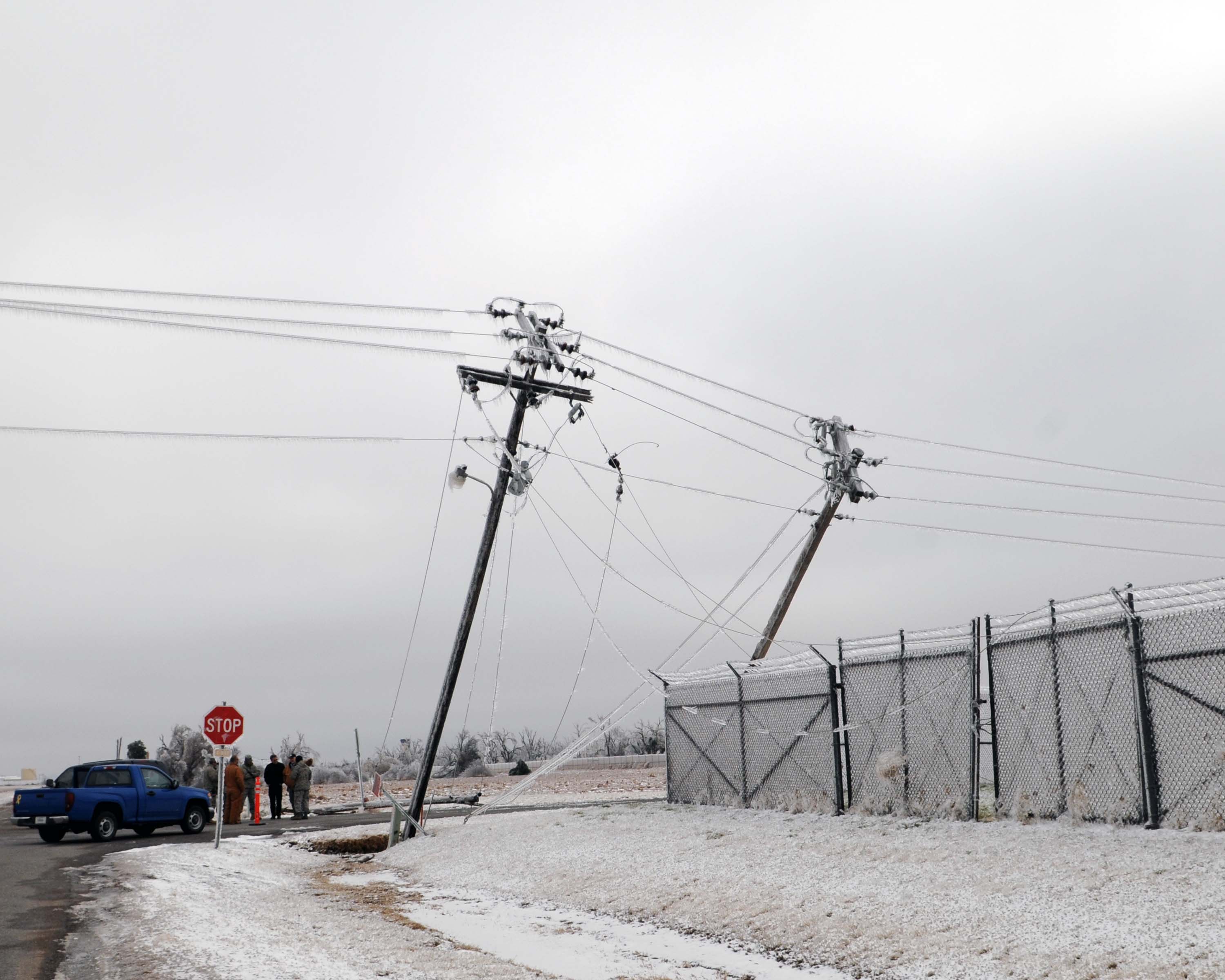
Weather conditions (hurricane, lightning, blizzard, flood, severe wind etc.), equipment failures due to component wearing or defective materials, accidents such as falling trees or car crashes on electricity poles and unpredictable events such as vandalism, hacking or equipment theft, are some of the causes of electricity interruptions.


And what can we do to restore power after a fault has occurred? The first step is to find where the fault occurred and what kind of fault occurred and then send a crew to fix the problem.
B) Fault detection, isolation and restoration
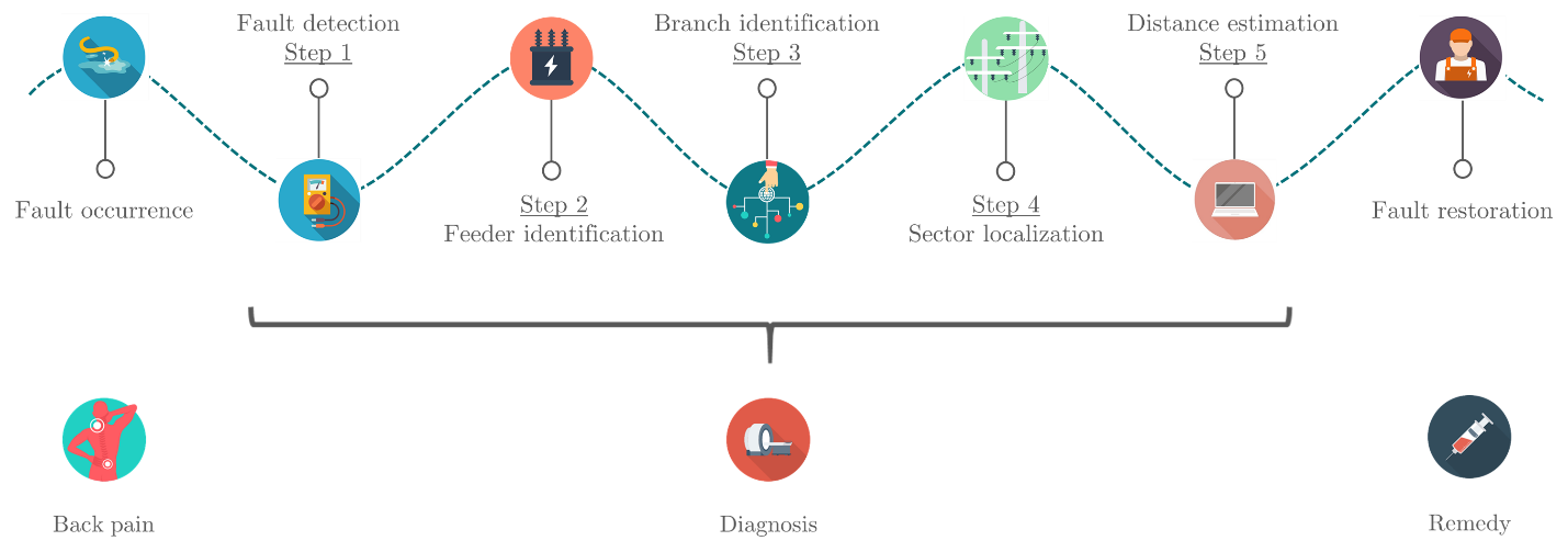
What would you do if you had a sudden back pain? The first step would be to go to a doctor. The doctor would then use different tools such as physical examination or an MRI scan to provide you with a diagnosis. Finally, once the differential diagnosis is made, she will prescribe you a remedy.
In the same way, when a fault occurs in a distribution grid, a certain strategy is needed to deal with it. But before going into more details let us give the definition of some basic terms.
Fault detection is the process of recognizing that a fault occurred and that the grid is not operating as intended.
Fault isolation is the process of identifying the fault, e.g. what kind of fault has occurred, and localizing it, e.g. finding where exactly it happened.
Fault diagnosis is the combined effort of both fault detection and isolation.
Fault restoration is the process of reconfiguration of the grid that is set in action after fault diagnosis in order for the grid to return back to its normal operating conditions.
At this point we should outline that even today, many distribution grid operators rely on customer phone calls to detect and localize a fault. Once a fault is reported, they send a crew to locate it and fix it. This is a very time consuming process that might leave customers without power for several minutes or even hours. However, in this new era of digitalization where the concept of the smart grid is introduced [5], new solutions arise, proposing the automation of the fault detection, isolation and restoration processes and minimize human interference [6].
In this Virtual Lab, we will analyze a fault diagnosis method and the effect of fault resistance on detecting and localizing single phase to ground faults. When a single line to ground short circuit fault occurs, e.g. when a cable breaks and touches the ground, then the current of the line will flow through the fault connection from the cable to the ground. Depending on the nature of the fault and the object touching the cable, the fault resistance will vary. Different objects have different levels of electrical conductivity and thus different amounts of current would flow through them in case they touched an electricity cable.
For the purpose of this Virtual Lab, we will use the example of a low voltage radial semi-rural distribution grid of Portugal, provided by Efacec (a beneficiary partner of INCITE-ITN). A schematic of this grid is given in the first picture of the slideshow below. The single line diagram of this grid is presented in the second picture of the slideshow.
The grid consists of a total of 3 feeders, 9 branches and 32 sectors (33 nodes). A grid branch is a unique line path from the beginning of a feeder to a terminal node; for example, the 1st branch is the line from node 1 to node 29 and the 9th branch is the line from node 1 to node 32. The grid sector is defined as the section of the grid connecting two adjacent nodes; for example, a sector of the grid is the line between nodes 11 and 18 or another one between nodes 8 and 14. Use the slideshow to get a better grasp of the notions of branch and sector.


The grid is completely heterogeneous, in the sense that the cables connecting the different sectors are of different type, presenting a big variety of resistances, reactances and lengths. This gird is also unbalanced since loads and micro-generation units, in this case photovoltaic installations of different sizes, are spread asymmetrically in the three phases of the grid; notice how the different houses are of different sizes in the first picture of the slideshow. The grid is equipped with voltage sensors in every node and current sensors in the beginning of each feeder as shown in the single line diagram of the grid.
Now that we have given the basic notions of the grid let us explore the fault diagnosis method. In the following picture, we can see the chain of events of the proposed strategy that follows a fault occurrence. As explained before, the fault diagnosis is divided in two categories: a) the fault detection (Steps 1-2) and b) the fault isolation (Steps 3-5).
- Fault detection
Step 1: Fault detection
Theoretically, at the moment of a fault occurrence a sudden increase of the current at the beginning of the feeder is expected.
In the following graph you can see the increase of the current during a fault as measured at the beginning of the feeder, in the per unit system (fault current divided by normal operation current measured 5 min before the fault occurrence). Attention! The following graph shows how a fault affects the current of the feeder to which it belongs and not how one fault affects the currents of all the feeders. For example, a fault with 0.1 Ω (Ohms) of fault resistance in the first feeder will cause an increase of the current by 11.97 times while a fault with the same fault resistance in the third feeder will cause an increase of the current by 24.2 times.
The influence of the fault resistance on the increase of the current is clearly depicted in the above graph. Use the slider to increase the fault resistance and notice how the increase of the fault resistance decreases the fault current. You can also click on the adjust button to re-scale the axis to the new values. For low fault resistance values (0.1 Ω) the fault current can be up to 25 times bigger, in terms of amplitude, than the one in normal operation; in the case of a fault in feeder 3, the measured fault current is 24.3 times bigger than the one in normal operation 5 minutes before the fault occurrence. On the other hand, for fault resistance values higher than 50 Ω, the fault current is slightly higher than the one observed in normal operation (values very close to 1 p.u.). This means that the occurrence of a fault can go undetected posing a huge threat to the grid. There are however, specialized detection techniques for high resistance faults thus making it possible to raise an alarm signal after their occurrence. But going into more details on this subject, is out of the scope of this virtual lab.
By now, you should be wondering why the three feeders do not present a similar behavior in terms of the observed fault current increase. This is explained by the heterogeneous and unbalanced nature of the grid, as it was described above. To understand this phenomenon easier, following the same analogy as before, imagine how different people perceive and tolerate in a different way a back pain.
Step 2: Faulty feeder identification
The identification of the feeder under fault is simply achieved by comparing the currents at the beginning of each feeder. The feeder that shows an increase in the current in any of each phases is considered as the one under faults.
- Fault isolation
Once the fault has been detected and the faulty feeder has been identified, an attempt should be made to localize the fault. Five big categories of fault location methods are reported in the literature: a) impedance based methods, b) traveling wave methods, c) methods using artificial intelligence and neural networks, d) methods based on voltage and current measurements and e) hybrid methods combining two or more of the above.
In this Virtual Lab we will examine a different fault isolation technique that is based on a voltage profile analysis across a faulty branch.
Step 3: Faulty branch identification
As shown in Fig. 2, the faulty branch identification is the first step of the fault isolation process (Step 3 of the fault diagnosis). Identifying which of the branches is under fault inside a feeder is done by using a simple criterion: the branch with the highest voltage drop is the one considered to be under fault. However, with the increase of fault resistance to higher values, the voltage drop becomes comparable with a drop that could be part of the normal grid operation. According to the EN50160 standard in LV grids, only a voltage drop higher than 10% of the one under normal operating conditions is considered as an anomaly.
Step 4: Faulty sector localization
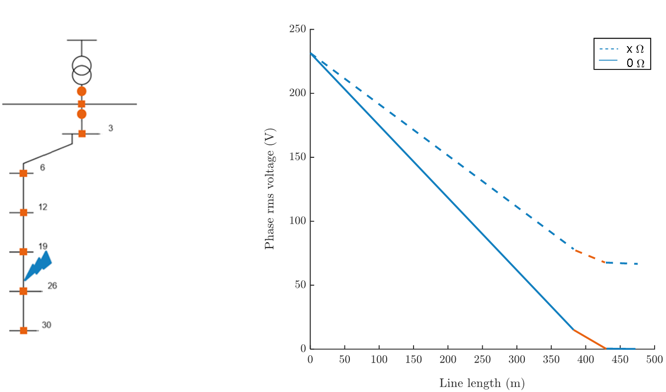
Following the faulty branch identification step, the faulty sector localization is launched. The idea of this method is based on the fact that a fault induces a voltage drop across the faulty branch. In fact, with zero fault resistance the voltage would drop to zero since all the current would flow from the faulty line to the ground. But this is almost never the case. For non-zero fault resistance values the voltage after the fault point instead of remaining zero would stabilize to a certain value. This stabilization means that the slope of the curve will come very close to zero and this is the characteristic that is being used to detect the faulty sector. The previous sector of the one where the voltage stabilizes is the one under fault. The above phenomenon is shown in the following figure where the faulty sector (19-26) is the orange one. Notice how theoretically we would expect the voltage to stabilize after the faulty sector.
Step 5: Fault distance estimation
The last step in localizing the fault, after identifying the faulty branch and sector, is to estimate its location within the faulty sector. To achieve that, a graphic method is implemented. From the linearly interpolated curve of the voltage measurement datapoints, the lines of the sectors adjacent to the one under fault are linearly extrapolated (green dashed lines) and their intersection point was used to estimate the location of the fault inside the sector.
To showcase the above process a slideshow with an example of a fault between nodes 9 and 16 of branch 1 is displayed below.
1 / 6 Linear interpolation between the measurement point to obtain the voltage profile accross a faulty branch.2 / 6
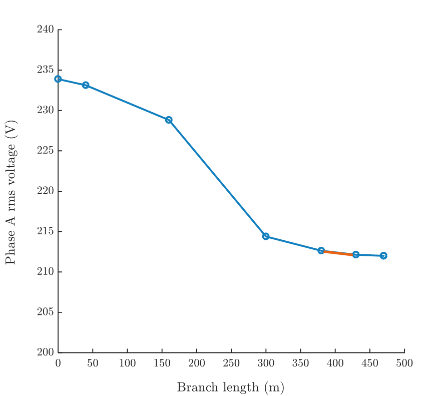 Faulty sector3 / 6
 Extrapolation of the curve from adjacent to the faulty, sectors4 / 6
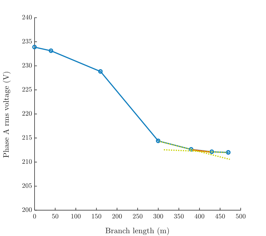 Extrapolation of the curve from adjacent to the faulty, sectors5 / 6
 Intersection point of the extrapolated lines❮ ❯6 / 6
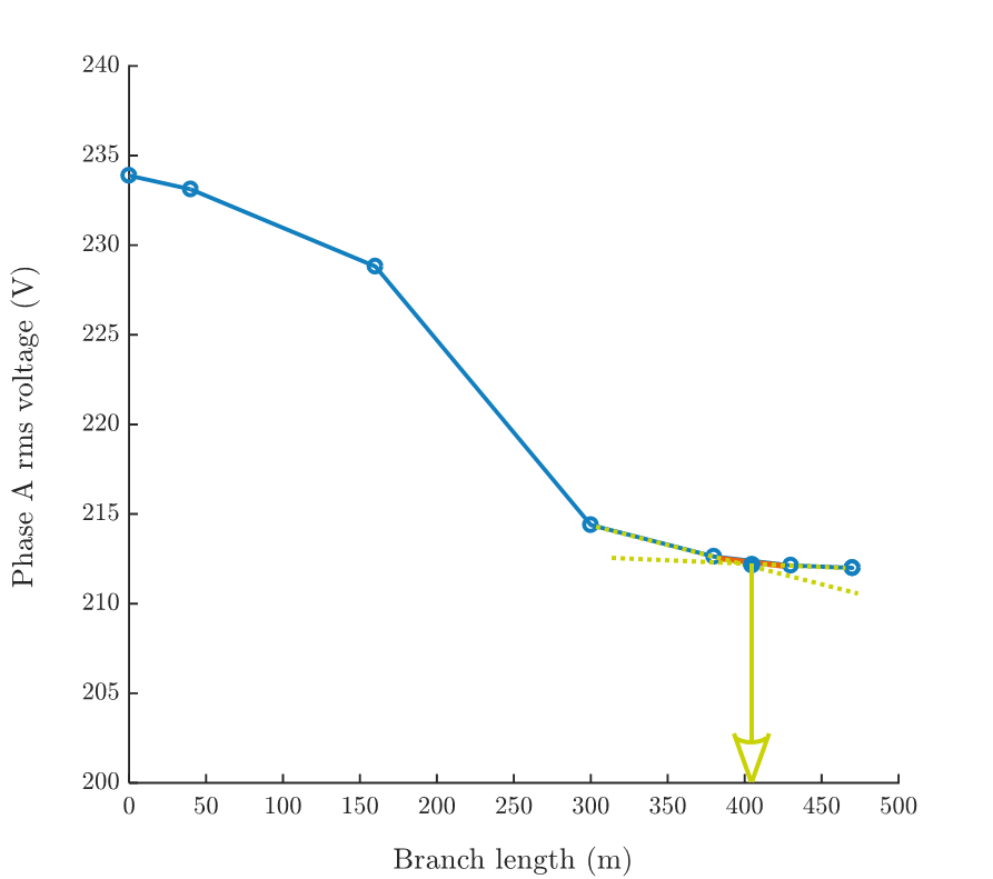 Fault location estimation
- Measuring tools
There are two available tools that we can use to monitor the voltage at every node.
Phase rms measurements:
The root mean square (rms) voltage of each phase is measured. Use the slider in the following curve to notice again how the increase of fault resistance affects the voltage profile along a faulty branch. Don't forget to use the auto-scale button!
Symmetrical component analysis:
A transformation of an electrical variable (current, voltage) is quite common in electrical engineering. The transformation often called symmetrical component analysis takes into account the measurements from each phase and creates three vectors: positive, negative and zero sequence components, each one of them containing information from every phase. The mathematical analysis of this process is however, out of scope of this VL.
Notice how the use of the positive sequence component of the voltage mitigates the effect of voltage drop for low fault resistance values. This happens for single phase to ground faults where only one phase is under fault; since the other two phases are not under fault, the value of the positive sequence component of the voltage will be higher from the value of the one at the faulty phase.
For more detailed information about the methods presented in this Virtual Lab follow the publication of ESR4.2, Nikolaos Sapountzoglou, in the 13th IEEE PowerTech conference.
References
[1] P. Linares and L. Rey, “The costs of electricity interruptions in Spain. Are we sending the right signals?,” Energy Policy, vol. 61, pp. 751–760, Oct. 2013.
[2] R. Isermann, Fault-diagnosis applications: model-based condition monitoring: actuators, drives, machinery, plants, sensors, and fault-tolerant systems. Berlin: Springer, 2011.
[3] T. Gönen, Electric Power Distribution Engineering, Third edition. Boca Raton: Taylor & Francis, 2014.
[4] CEER, “6th Benchmarking Report on the Continuity of Electricity and Gas Supply,” Brussels, C 18-EQS-86-03, 2016.
[5] N. Sapountzoglou, "Solar energy: The once and future King"
[6] A. Zidan et al., “Fault Detection, Isolation, and Service Restoration in Distribution Systems: State-of-the-Art and Future Trends,” IEEE Trans. Smart Grid, vol. 8, no. 5, pp. 2170–2185, Sep. 2017.


© 2019, Nikolaos Sapountzoglou.Special thanks to Mr. George Bouzias and Mr. Felix Koeth for their useful insights and feedback.Icons made by Freepik, Icon Pond, DinosoftLabs and Vectors Market from www.flaticon.com is licensed by CC 3.0 BY. Icons were also designed by macrovector, macrovector_official / Freepik.Released under a license.
- Measuring tools